_-_Galton_1889_diagram.png.webp)

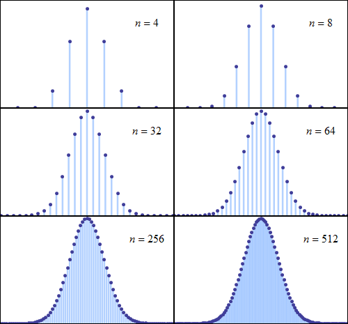
In probability theory, the de Moivre–Laplace theorem, which is a special case of the central limit theorem, states that the normal distribution may be used as an approximation to the binomial distribution under certain conditions. In particular, the theorem shows that the probability mass function of the random number of "successes" observed in a series of independent Bernoulli trials, each having probability of success (a binomial distribution with trials), converges to the probability density function of the normal distribution with mean and standard deviation , as grows large, assuming is not or .
The theorem appeared in the second edition of The Doctrine of Chances by Abraham de Moivre, published in 1738. Although de Moivre did not use the term "Bernoulli trials", he wrote about the probability distribution of the number of times "heads" appears when a coin is tossed 3600 times.[1]
This is one derivation of the particular Gaussian function used in the normal distribution.
It is a special case of the central limit theorem because a Bernoulli process can be thought of as the drawing of independent random variables from a bimodal discrete distribution with non-zero probability only for values 0 and 1. In this case, the binomial distribution models the number of successes (i.e., the number of 1s), whereas the central limit theorem states that, given sufficiently large n, the distribution of the sample means will be approximately normal. However, because in this case the fraction of successes (i.e., the number of 1s divided by the number of trials, n) is equal to the sample mean, the distribution of the fractions of successes (described by the binomial distribution divided by the constant n) and the distribution of the sample means (approximately normal with large n due to the central limit theorem) are equivalent.
Theorem
As n grows large, for k in the neighborhood of np we can approximate[2][3]
in the sense that the ratio of the left-hand side to the right-hand side converges to 1 as n → ∞.
Proof
The theorem can be more rigorously stated as follows: , with a binomially distributed random variable, approaches the standard normal as , with the ratio of the probability mass of to the limiting normal density being 1. This can be shown for an arbitrary nonzero and finite point . On the unscaled curve for , this would be a point given by
For example, with at 3, stays 3 standard deviations from the mean in the unscaled curve.
The normal distribution with mean and standard deviation is defined by the differential equation (DE)
- with an initial condition set by the probability axiom .
The binomial distribution limit approaches the normal if the binomial satisfies this DE. As the binomial is discrete the equation starts as a difference equation whose limit morphs to a DE. Difference equations use the discrete derivative, , the change for step size 1. As , the discrete derivative becomes the continuous derivative. Hence the proof need show only that, for the unscaled binomial distribution,
- as .
The required result can be shown directly:
The last holds because the term dominates both the denominator and the numerator as .
As takes just integral values, the constant is subject to a rounding error. However, the maximum of this error, , is a vanishing value.[4]
Alternative proof
The proof consists of transforming the left-hand side (in the statement of the theorem) to the right-hand side by three approximations.
First, according to Stirling's formula, the factorial of a large number n can be replaced with the approximation
Thus
Next, the approximation is used to match the root above to the desired root on the right-hand side.
Finally, the expression is rewritten as an exponential and the Taylor Series approximation for ln(1+x) is used:
Then
Each "" in the above argument is a statement that two quantities are asymptotically equivalent as n increases, in the same sense as in the original statement of the theorem—i.e., that the ratio of each pair of quantities approaches 1 as n → ∞.
See also
- Poisson limit theorem an alternative approximation of the binomial distribution for large values of n.
Notes
- ↑ Walker, Helen M (1985). "De Moivre on the law of normal probability" (PDF). In Smith, David Eugene (ed.). A source book in mathematics. Dover. p. 78. ISBN 0-486-64690-4.
But altho' the taking an infinite number of Experiments be not practicable, yet the preceding Conclusions may very well be applied to finite numbers, provided they be great, for Instance, if 3600 Experiments be taken, make n = 3600, hence ½n will be = 1800, and ½√n 30, then the Probability of the Event's neither appearing oftner than 1830 times, nor more rarely than 1770, will be 0.682688.
- ↑ Papoulis, Athanasios; Pillai, S. Unnikrishna (2002). Probability, Random Variables, and Stochastic Processes (4th ed.). Boston: McGraw-Hill. ISBN 0-07-122661-3.
- ↑ Feller, W. (1968). An Introduction to Probability Theory and Its Applications. Vol. 1. Wiley. Section VII.3. ISBN 0-471-25708-7.
- ↑ Thamattoor, Ajoy (2018). "Normal limit of the binomial via the discrete derivative". The College Mathematics Journal. 49 (3): 216–217. doi:10.1080/07468342.2018.1440872. S2CID 125977913.