Lattice model (physics)

A three-dimensional lattice filled with two molecules A and B, here shown as black and white spheres. Lattices such as this are used - for example - in the Flory–Huggins solution theory

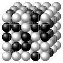
In mathematical physics, a lattice model is a mathematical model of a physical system that is defined on a lattice, as opposed to a continuum, such as the continuum of space or spacetime. Lattice models originally occurred in the context of condensed matter physics, where the atoms of a crystal automatically form a lattice. Currently, lattice models are quite popular in theoretical physics, for many reasons. Some models are exactly solvable, and thus offer insight into physics beyond what can be learned from perturbation theory. Lattice models are also ideal for study by the methods of computational physics, as the discretization of any continuum model automatically turns it into a lattice model. The exact solution to many of these models (when they are solvable) includes the presence of solitons. Techniques for solving these include the inverse scattering transform and the method of Lax pairs, the Yang–Baxter equation and quantum groups. The solution of these models has given insights into the nature of phase transitions, magnetization and scaling behaviour, as well as insights into the nature of quantum field theory. Physical lattice models frequently occur as an approximation to a continuum theory, either to give an ultraviolet cutoff to the theory to prevent divergences or to perform numerical computations. An example of a continuum theory that is widely studied by lattice models is the QCD lattice model, a discretization of quantum chromodynamics. However, digital physics considers nature fundamentally discrete at the Planck scale, which imposes upper limit to the density of information, aka Holographic principle. More generally, lattice gauge theory and lattice field theory are areas of study. Lattice models are also used to simulate the structure and dynamics of polymers.

Mathematical description

A number of lattice models can be described by the following data:

A lattice $\Lambda$ , often taken to be a lattice in $d$ -dimensional Euclidean space $\mathbb {R} ^{d}$ or the $d$ -dimensional torus if the lattice is periodic. Concretely, $\Lambda$ is often the cubic lattice. If two points on the lattice are considered 'nearest neighbours', then they can be connected by an edge, turning the lattice into a lattice graph. The vertices of $\Lambda$ are sometimes referred to as sites.
A spin-variable space $S$ . The configuration space ${\mathcal {C}}$ of possible system states is then the space of functions ${\displaystyle \sigma$ . For some models, we might instead consider instead the space of functions $\sigma :E\rightarrow S$ where $E$ is the edge set of the graph defined above.
An energy functional $E:{\mathcal {C}}\rightarrow \mathbb {R}$ , which might depend on a set of additional parameters or 'coupling constants' $\{g_{i}\}$ .

Examples

The Ising model is given by the usual cubic lattice graph $G=(\Lambda ,E)$ where $\Lambda$ is an infinite cubic lattice in $\mathbb {R} ^{d}$ or a period $n$ cubic lattice in $T^{d}$ , and $E$ is the edge set of nearest neighbours (the same letter is used for the energy functional but the different usages are distinguishable based on context). The spin-variable space is $S=\{+1,-1\}=\mathbb {Z} _{2}$ . The energy functional is

E(\sigma )=-H\sum _{v\in \Lambda }\sigma (v)-J\sum _{\{v_{1},v_{2}\}\in E}\sigma (v_{1})\sigma (v_{2}).

The spin-variable space can often be described as a coset. For example, for the Potts model we have $S=\mathbb {Z} _{n}$ . In the limit $n\rightarrow \infty$ , we obtain the XY model which has $S=SO(2)$ . Generalising the XY model to higher dimensions gives the $n$ -vector model which has $S=S^{n}=SO(n+1)/SO(n)$ .

Solvable models

We specialise to a lattice with a finite number of points, and a finite spin-variable space. This can be achieved by making the lattice periodic, with period $n$ in $d$ dimensions. Then the configuration space ${\mathcal {C}}$ is also finite. We can define the partition function

Z=\sum _{\sigma \in {\mathcal {C}}}\exp(-\beta E(\sigma ))

and there are no issues of convergence (like those which emerge in field theory) since the sum is finite. In theory, this sum can be computed to obtain an expression which is dependent only on the parameters $\{g_{i}\}$ and $\beta$ . In practice, this is often difficult due to non-linear interactions between sites. Models with a closed-form expression for the partition function are known as exactly solvable.

Examples of exactly solvable models are the periodic 1D Ising model, and the periodic 2D Ising model with vanishing external magnetic field, $H=0,$ but for dimension $d>2$ , the Ising model remains unsolved.

Mean field theory

Due to the difficulty of deriving exact solutions, in order to obtain analytic results we often must resort to mean field theory. This mean field may be spatially varying, or global.

Global mean field

The configuration space ${\mathcal {C}}$ of functions $\sigma$ is replaced by the convex hull of the spin space $S$ , when $S$ has a realisation in terms of a subset of $\mathbb {R} ^{m}$ . We'll denote this by $\langle {\mathcal {C}}\rangle$ . This arises as in going to the mean value of the field, we have ${\displaystyle \sigma \mapsto \langle \sigma \rangle$ .

As the number of lattice sites $N=|\Lambda |\rightarrow \infty$ , the possible values of $\langle \sigma \rangle$ fill out the convex hull of $S$ . By making a suitable approximation, the energy functional becomes a function of the mean field, that is, $E(\sigma )\mapsto E(\langle \sigma \rangle ).$ The partition function then becomes

Z=\int _{\langle {\mathcal {C}}\rangle }d\langle \sigma \rangle e^{-\beta E(\langle \sigma \rangle )}\Omega (\langle \sigma \rangle )=:\int _{\langle {\mathcal {C}}\rangle }d\langle \sigma \rangle e^{-N\beta f(\langle \sigma \rangle )}.

As $N\rightarrow \infty$ , that is, in the thermodynamic limit, the saddle point approximation tells us the integral is asymptotically dominated by the value at which $f(\langle \sigma \rangle )$ is minimised:

Z\sim e^{-N\beta f(\langle \sigma \rangle _{0})}

where $\langle \sigma \rangle _{0}$ is the argument minimising $f$ .

A simpler, but less mathematically rigorous approach which nevertheless sometimes gives correct results comes from linearising the theory about the mean field $\langle \sigma \rangle$ . Writing configurations as $\sigma (v)=\langle \sigma \rangle +\Delta \sigma (v)$ , truncating terms of ${\mathcal {O}}(\Delta \sigma ^{2})$ then summing over configurations allows computation of the partition function.

Such an approach to the periodic Ising model in $d$ dimensions provides insight into phase transitions.

Spatially varying mean field

Suppose the continuum limit of the lattice $\Lambda$ is $\mathbb {R} ^{d}$ . Instead of averaging over all of $\Lambda$ , we average over neighbourhoods of $\mathbf {x} \in \mathbb {R} ^{d}$ . This gives a spatially varying mean field ${\displaystyle \langle \sigma \rangle$ . We relabel $\langle \sigma \rangle$ with $\phi$ to bring the notation closer to field theory. This allows the partition function to be written as a path integral

Z=\int {\mathcal {D}}\phi e^{-\beta F[\phi ]}

where the free energy $F[\phi ]$ is a Wick rotated version of the action in quantum field theory.

Examples

Condensed matter physics

Polymer physics

Bond fluctuation model
2nd model

High energy physics

QCD lattice model

References

Baxter, Rodney J. (1982), Exactly solved models in statistical mechanics (PDF), London: Academic Press Inc. [Harcourt Brace Jovanovich Publishers], ISBN 978-0-12-083180-7, MR 0690578

This article is issued from Wikipedia. The text is licensed under Creative Commons - Attribution - Sharealike. Additional terms may apply for the media files.

Mathematical description

Examples

Solvable models

Mean field theory

Global mean field

Spatially varying mean field

Examples

Condensed matter physics

Polymer physics

High energy physics

See also

References